Infinite-ISP Tutorial: Salient Features

Now that we’ve covered the fundamentals, let’s delve further into the Infinite-ISP open-source repository to uncover even more of its extensive features. This tutorial will walk you through various image processing tasks, including the configuration of Infinite-ISP class using customized or default parameter configuration for dataset or video processing, as well as enhancing image quality through the utilization of 2A modules.

Follow along to learn more on the following aspects of Infinite-ISP:

How to process an image using render-3a feature
How to process a dataset using Infinite-ISP pipeline
How to apply video processing on a set of images
How to generate test vectors using automation script

Github Repository: Reference Model Infinite-ISP_AlgorithmDesign

Note: The features listed above are available in both Reference Model and Infinite-ISP_AlgorithmDesign except for the last feature enabling test vector generation and is only available in the Reference Model.

Exploring the Getting started with Infinite ISP section is encouraged for individuals seeking a solid grasp of the basics of Infinite-ISP.

How to process an image using render-3A feature

What is 3A?

In an ISP, 3A refers to the three modules namely auto white balance (AWB), auto exposure (AE) and auto focus (AF, not currently implemented in infinite ISP), which significantly contribute to the quality of the image an ISP delivers. AWB aims to achieve a natural-looking coloration in the output image whereas AE corrects the brightness of the captured scene by applying digital gain. AF adjusts the focus to achieve best contrast ensuring that the contents of the image appear clear and well-defined.

It would be a good exercise for you to pause and observe the image quality degradation by switching off white balance by setting the is_enable flag to False

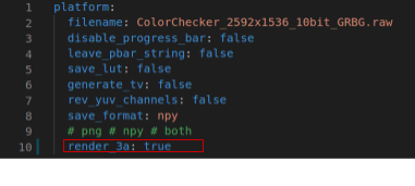
The 3A render feature updates digital gain and white balance gains in the config file based on feedback and reruns the pipeline. This process continues until the parameters are approved by the 2A modules or they can no longer be improved. The user can enable this feature in the config file using the render_3a flag as indicated in the image below.

The final output of the very last iteration is saved in the ./out_frames directory.

2A in Infinite-ISP

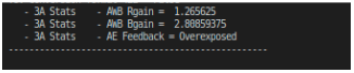
Infinite-ISP has a special feature that enables 2 of the 3A modules (AE and AWB, AF will be implemented soon). It simulates the actual working of the 3A blocks in an ISP using the 3A rendering feature. Infinite-ISP implements 2A modules as a frame pass algorithm to fine-tune the respective parameters for optimal image quality based on 2A stats computed at various points/locations in the pipeline. The InfiniteISP class computes the 2A stats on the input image iteratively and applies them to the same image in the following iteration after tweaking them based on the provided feedback. This feedback can be found at the very end of the printed logs as shown in the image below. For example, in the getting started tutorial, the AE feedback says “overexposed” indicating that image quality can be improved by reducing the digital gain applied (if possible). Similarly, AWB provides a better estimate of the R and B gain parameters.

Example

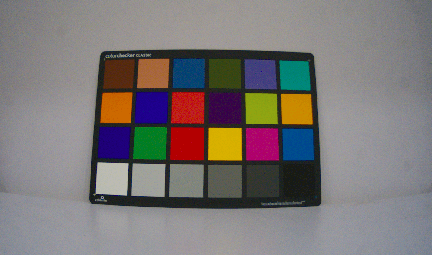
We will be using the sample raw image ColorChecker_2592x1536_10bit_GRBG from the ./in_frame/normal directory, along with the default configuration file from the ./config directory.

Because the parameters in the config file are already tuned for the provided input image, let’s tweak them a little to produce inaccurate results first. This can be easily done by changing the configuration parameters as follows.

Go to configs.yml in ./config directory
Set render_3a flag to false
Set the R and B gains to 1
Set the current_gain parameter to 3 under the digital gain heading
Run ./isp_pipeline.py file

Now let us enable the 2A modules in the pipeline and compare the results. For this, enable image rendering with the same parameter configuration to see the render-3A feature in action.

For this

Go to configs.yml in ./config directory
Set render_3a flag to true
Set the R and B gains to 1
Set the current_gain parameter to 3 under the digital gain heading
Run ./isp_pipeline.py file

The results presented below clearly demonstrate the significance of parameter tuning in raw image processing.

The 3A render feature adjusts the digital gain and WB gains in each consecutive run until no further improvement can be made. The image below demonstrates how these updations can be tracked using the output logs printed in the terminal.

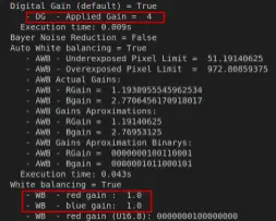
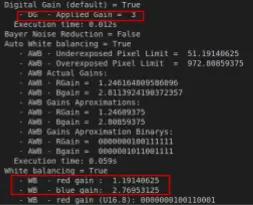
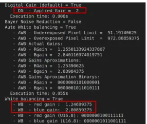
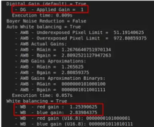
Image Rendering Logs

The output image is returned once no improvement is observed in parameter estimation.

How to process a dataset using Infinite-ISP pipeline

You can use an Infinite-ISP pipeline to process an entire dataset as a whole. Currently three file formats are supported by the infinite-ISP pipeline namely .raw, .NEF and .dng. While processing files other than .raw files the sensor specific information, such as image dimension, bayer pattern and bit depth, is extracted from the image metadata and is automatically updated in the config file under sensor_info heading.

Dataset

Your dataset is a directory containing some input files (with supported file formats). You can either process this data using the same parameter configuration for all input files or provide a custom parameter configuration for each of the input files. For the former task, simply update the default config provided in the ./config directory. However, for the later task, you can follow the steps given below to create an image-specific config file.

Copy the default config file in your data directory
Rename the config file as: <img_name>-configs
Update the parameter configuration according to the image

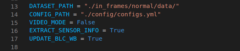
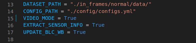
The script ./isp_pipeline_multiple_images.py has already been configured to process the sample data provided in ./in_frames/data directory but you can also configure the variable in the python script ./isp_pipeline_multiple_images.py to process a dataset on your local computer as explained below.

Configure script parameters

Update the DATASET_PATH variable by providing the absolute path in order to process a local dataset. The CONFIG_PATH variable defines your default configuration which is used in case an image-specific config file is not provided with the image. Set video mode to false to process each image independently.

Dataset as a submodule

If your dataset is present on another git repository you can use it as a submodule by following the steps below.

Open terminal and navigate to the cloned Infinite ISP repo.

cd <path_to_ISP_repo>

Add you dataset as a submodule

git submodule add <url> <path>

Up your date and initialize submodule

git submodule update --init--recursive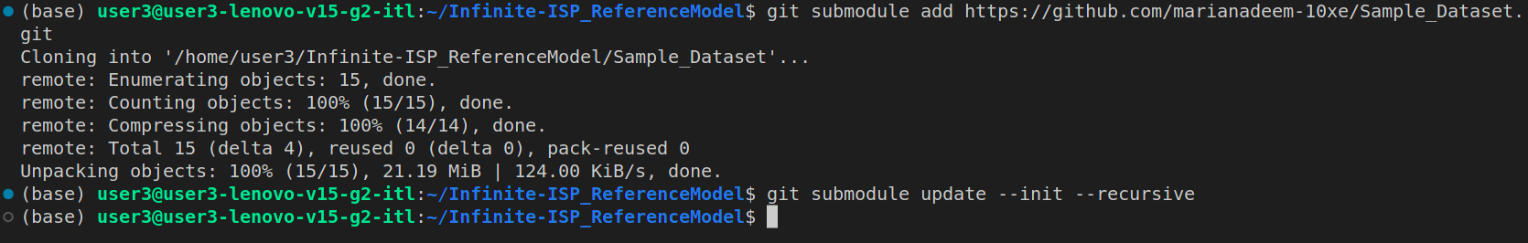

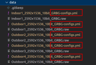
Now that you have successfully initialized your submodule, you are ready to process your dataset. Make sure to rename the config files, in the dataset, by appending the “-configs” tag at the end as shown below.

Lastly, Configure the script parameters accordingly and you are good to go!

Execute python script

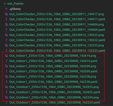
Now simply run the isp_pipeline_multiple_images.py file. Upon execution, the generated output files are placed in the ./out_frames directory along with a copy of the config file used to generate the resultant image.

Working

The script iteratively processes each input file looking for a corresponding config file named <imagename>-configs.yml for each raw file. When a custom config file is not provided in the dataset, it falls back to utilizing the default config file. If single parameter configuration is used for all the input files i.e. using a single config file to process all input files, the code automatically updates the file-specified parameters in the config. For example, the file name is updated for .raw files and sensor info, BLC, and WB parameters are updated for .NEF and .dng files.

Tip: To save yourself from tuning the gain parameters for each image while processing a dataset, just enable the render-3A flag!

How to apply video processing on a set of images

The video mode works in a very similar manner as the render-3A feature. The only difference is that the feedback provided for one frame is applied onto the next frame, processing each frame only once. As a video is a set of frames captured in sequence, a single config file is used. One thing you have to keep in mind is to order your raw files by appending numerical tags at the end of the filename e.g. <filename>_001. Enable the video mode in the isp_pipeline_multiple_images.py file and run it.

The output files can be accessed in the ./out_frames directory.

How to generate test vectors using automation script

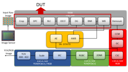
The ./test_vector_generation directory is specifically designed to test and debug a specific part of the pipeline. This feature can be used to tap output from any point of the pipeline by defining that part as device under test (DUT) which can be a single module or a set of consecutive modules. Let’s demonstrate with an example to get a clear picture. Say, you want to test the part of the pipeline which processes the raw data (red box in the image below) i.e before the application of color filter array (CFA) which interpolates the raw data to create the 3-channel RGB image.

1. Configure paths

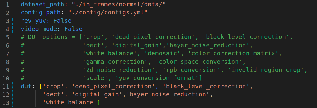
Firstly, go to the ./test_vector_generation directory and set the dataset and default configuration paths and the video mode flag, in the ./test_vector_generation/tv_config file, just like you configured in case of dataset and video processing. The rev_yuv flag is explained later in this tutorial and is kept disabled for now.

2. Define DUT list

Next, choose your DUT from the provided list of options. Simply copy and paste the specific part of the pipeline that you want to test. Make sure you don’t change the format of the module names, as they are used to update the config files to adjust settings according to your preferences.

3. Define pipeline configuration

Lastly, you can enable / disable any other modules excluding the ones set as DUT because these modules are enabled automatically by the automation script.

Note that the default modules, namely digital gain, demosaic, and color space conversion, use the “is_save” flag instead of “is_enable.” This is because default modules cannot be disabled.

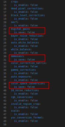
For all modules in the DUT list, the “is_save” flag is automatically enabled. However, if you want to save the output files for the modules other than the ones defined as DUT, you need to manually enable the “is_save” flag in tv_config, for the default modules, or in the image config, for non-default modules.

4. Execute script

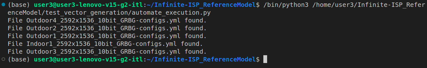
Alright! you are all set to run the automation script. By executing the script for the provided sample data in ./in_frames/data directory, the following is what you see as the terminal output. This shows that each image was processed using its respective config file as provided in the data folder.

The results are saved in the ./test_vectors directory, which is created on run time, with a datetime stamp.

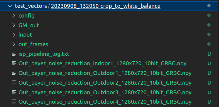
These results include the following files and directories:

config (directory): contains the updated config files used to generate these results.
GM_out (directory): output array (.npy files) of the last module in DUT
input (directory): input array (.npy, .bin files) to the first module in DUT list, input of crop module in this example
out_frames (directory): pipeline output files (.png or .npy acc. To the save_format parameter)
isp_pipeline_log (text file): Terminal output briefing pipeline configuration
tv_config (yaml file): copy of the tv_config used
30 numpy arrays (.npy files): output of each intermediate module for 5 images (5×6).

Rev_yuv Flag

The automation script saves the input arrays to DUT as a single binary file in case of a raw image (as in this example) and saves three binary files for a 3-channel RGB image with respective channel tags added in the beginning of the binary filenames. In case of a YUV image (e.g. last module in DUT is 2DNR), Y channel is always saved with “B” tag, U with “G” tag and V with “R” tag in the input directory of the generated results. The rev_yuv flag in the tv_config allows you to reverse this order.

You can use the render_3a or the video_mode flags as previously explained. Please refer to the ./doc directory and README files for detailed information.

Conclusion

As we conclude this tutorial, you’ve acquired significant insight into Infinite-ISP’s amazing image processing capabilities. However, guess what? There’s even more to discover! In our next content, we’ll go into greater detail on how to use our open-source ISP as your creative sandbox. Stay tuned for fascinating new chapters in our exploration.